| Time to Delivery | Hour of Order | Day of Order | Distance |
Item Counts
|
|||
|---|---|---|---|---|---|---|---|
| 1 | 2 | ... | 27 | ||||
| 15.26 | 11.9 | Thu | 2.82 | 0 | 0 | ... | 0 |
| 27.45 | 19.2 | Wed | 3.59 | 0 | 0 | ... | 1 |
| 25.50 | 14.9 | Thu | 2.28 | 2 | 0 | ... | 0 |
| 17.34 | 12.2 | Wed | 3.26 | 0 | 0 | ... | 0 |
| 13.58 | 11.5 | Fri | 2.15 | 2 | 0 | ... | 0 |
| 25.55 | 15.4 | Sat | 2.17 | 0 | 0 | ... | 0 |
| 19.86 | 13.2 | Tue | 2.67 | 0 | 0 | ... | 0 |
| 28.25 | 15.7 | Sun | 4.24 | 1 | 0 | ... | 1 |
1 Introduction
Machine learning (ML) models are mathematical equations that take inputs, called predictors, and try to estimate some future output value. The output, often called an outcome or target, can be numbers, categories, or other types of values.
For example, in the next chapter, we try to predict how long it takes to deliver food ordered from a restaurant. The outcome is the time from the initial order (in minutes). There are multiple predictors, including: the distance from the restaurant to the delivery location, the date/time of the order, and which items were included in the order. These data are tabular; they can be arranged in a table-like way (such as a spreadsheet or database table) where variables are arranged in columns and individual data points (i.e., instances of food orders) in rows, as shown in Table 1.11.
Note that the predictor values are almost always known. For future data, the outcome is not; it is a machine learning model’s job to predict unknown outcome values.
How does it do that? A specific machine learning model has a defined mathematical prediction equation defining exactly how the predictors relate to the outcome. We’ll see two very different prediction equations shortly.
The prediction equation includes some unknown parameters. These are placeholders for values that help us best predict the outcomes. The process of model training (also called “fitting” or “estimation”) takes our existing predictor and outcome data and uses them to find the “optimal” values of these unknown parameters. Once we estimate these unknowns, we can use them and specific predictor values to estimate future outcome values.
Here is a simple example of a prediction equation with a single predictor (the distance) and two unknown parameters that have been estimated:
delivery\:time = \exp\left[2.944 + 0.096 \: distance\right] \tag{1.1}
We could use this equation for new orders:
- If we had placed an order at the restaurant (i.e., a zero distance) we predict that it would take e^{2.944} \approx 19 minutes.
- If we were four miles away, the predicted delivery time is e^{(2.944 + 0.382)} \approx 27.85 minutes.
and so on.
This is an incredibly reductive approach; it assumes that the relationship between the distance and time are log-linearly related and is not influenced by any other characteristics of the process. On the bright side, the exponential function ensures that there are no negative time predictions, and it is straightforward to explain.
How did we arrive at values of 2.944 and 0.096? They were estimated from data once we made a few assumptions about our model. We started off by proposing a format for the prediction equation: an additive, log-linear function2 that includes unknown parameters \beta_0 and \beta_1:
{ \color{darkseagreen} \underbrace{\color{black} log(time)}_{\text{the outcome}} } = { \color{darkseagreen} \overbrace{\color{black} \beta_0+\beta_1\, distance}^{\text{an additive function of the predictors}} } + { \color{darkseagreen} \underbrace{\color{black} \epsilon}_{\text{the errors}} }
To estimate the parameters, we chose some type of criterion to quantify what it means to be “good” values (called an objective function or performance metric). Here we will pick values of the \beta parameters that minimize the squared error, with the error (\epsilon) defined as the difference in the observed and predicted times (on the log scale).
Based on this criterion, we can define intermediate equations that, if we solve them, will result in the best possible parameter estimates given the data and our choices for the prediction equation and objective function.
Sadly, Equation 1.1, while better than a random guess, is not very effective. It does the best it can with a the single predictor. It just isn’t very accurate.
To illustrate the diversity of different ML models, Equation 1.2 shows a completely different kind of prediction equation. This was estimated from a model called a regression tree. The function I(\cdot) is one if the logical statement is true and zero otherwise. Two predictors (distance and day of the week) were used in this case.
\begin{align} time = \:&23.0\, I\left(distance < 4.465 \text{ miles and } day \in \{Mon, Tue, Wed, Sun\}\right) + \notag \\ \:&27.0\, I\left(distance < 4.465 \text{ miles and } day \in \{Thu, Fri, Sat\}\right) + \notag \\ \:&29.8\, I\left(distance \ge 4.465 \text{ miles and } day \in \{Mon, Tue, Wed, Sun\}\right) + \notag \\ \:&36.5\, I\left(distance \ge 4.465 \text{ miles and } day \in \{Thu, Fri, Sat\}\right)\notag \end{align} \tag{1.2}
A regression tree determines the best predictors(s) to “split” the data, making smaller and smaller subsets of the data. The goal is to make the subsets within each split have about the same outcome value. The coefficients for each logical group are the average of the delivery times for each subset defined by the statement with the I(\cdot) terms. Note that these logical statements, called rules, are mutually exclusive; only one of the four subsets will be true for any data point being predicted.
Like the linear regression model that produced Equation 1.1, the performance of Equation 1.2 is quite poor. There are only four possible predicted delivery times. This particular model is not known for its predictive ability, but it can be highly predictive when combined with other regression trees into an ensemble model.
This book is focused on the practice of applying various ML models to data to make accurate predictions. Before proceeding, we’ll discuss different types of the data used to estimate models and then explore some aspects of ML models, particularly neural networks.
1.1 Non-Tabular Data
The columns shown in Table 1.1 are defined within a small scope. For example, the delivery hour column encapsulates everything about that order characteristic:
- You don’t need any other columns to define it.
- A single number is all that is required to describe that information.
Non-tabular data does not have the same properties. Consider images, such as the one shown Figure 1.1 that depicts four cells from a biological experiment (Yu et al. 2007). These cells that have been stained with pigments that fluoresce at different wavelengths to “paint” different parts of the cells. In this image, blue reflects the part of the cell called the cytoskeleton, which encompasses the entire cell body. The red color corresponds to a stain that only attaches itself to the contents of the cell nucleus, specifically DNA. This image3 is 371 pixels by 341 pixels with quantification of two colors.
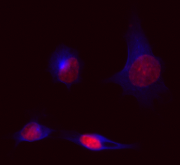
From a data perspective, this image is represented as a three-dimensional array (371 rows, 341 columns, and 2 colors). Probably the most important attribute of this data is the spatial relationships between pixels. It is critical to know where each value in the 3D array resides, but knowing what the nearby values are is at least as important.
We could “flatten” the array into 371 \times 341 \times 2 = 253,022 columns to use in a table4. However, this would break the spatial link between the data points; each column is no longer as self-contained as the columns from the delivery data. The result is that we have to consider the 3D array as the data instead of each row/column/color combination.
Additionally, images often have different dimensions which results in different array sizes. From a tabular data perspective, a flattened version of such data would have a different number of columns for different-sized images.
Videos are an extension of image data if we were to consider it a four-dimensional array (with time as the additional dimension). The temporal aspects of such data are critical to understanding and predicting values.
Text data are often thought of as non-tabular data. As an example, consider text from Sanderson (2017):
“The most important step a man can take. It’s not the first one, is it? It’s the next one. Always the next step, Dalinar.”
With text data, it is common to define the “token”: the unit of text that should be analyzed. This could be a paragraph, sentence, word, etc. Suppose that we used sentences as tokens. In this case, the table for this quote would have four rows. Where do we go from here? The sequence of words (or characters) is likely to be important, and this makes a case for keeping the sentences as strings. However, as will be seen shortly, we might be able to convert these four tokens to numeric columns in a way that preserves the information required for prediction.
Perhaps a better text example relates to the structure of chemicals. A chemical is a three-dimensional molecule but is often described using a SMILES string (Engel and Gasteiger 2018, chap. 3). This is a textual description of molecule that lists its elements and how they relate to one another. For example, the SMILES string CC(C)CC1=CC=C(C=C1)C(C)C(=O)O defines the anti-inflammatory drug Ibuprofen. The letters describe the elements (C is carbon, O is oxygen, etc) and the other characters defines the bonds between the elements. The character sequence within this string is critical to understanding the data.
Our motives for categorizing data as tabular and non-tabular are related to how we choose an appropriate model. Our opinion is that most modeling projects involve tabular data (or data that can be effectively represented as tabular). Models for non-tabular data are very specialized and, while these ML approaches are the most discussed in the social media, they tend not to be the best approach for tabular data.
1.2 Converting Non-Tabular Data to Tabular
In some situations, non-tabular data can be effectively converted to a tabular format, depending on the specific problem and data.
For some modeling projects using images, we might not be interested in every pixel. For Figure 1.1, we really care about the cells in the image. It is important to understand within-cell characteristics (e.g. shape or size) and some between-cell information (e.g., the distance between cells). The vast majority of the pixels don’t need to be analyzed.
We can pre-analyze the 3D arrays to determine which pixels in an image correspond to specific cells (or nuclei within a cell). Segmentation (Holmes and Huber 2018) is the process of estimating regions of an image that define some object(s). Figure 1.2 shows the same cells with lines generated from a simple segmentation.

Once our cells have been segmented, we can compute various statistics of interest based on size, shape, or color. If a cell is our unit of data, we can create a tabular format where rows are cells and columns are cell characteristics (Table 1.2). The result is a data table that has more rows than the original non-tabular structure since there are multiple cells in an image. There are far fewer columns but these columns are designed to be more informative than the raw pixel data since the researchers define the cell characteristics that they desire.
| ID |
Eccentricity
|
Area
|
Intensity
|
|||||
|---|---|---|---|---|---|---|---|---|
| Nucleus | Cell | Nucleus | Cell | Nucleus | Cell | |||
| 17 | 0.494 | 0.836 | 3,352 | 11,699 | 0.274 | 0.155 | ||
| 18 | 0.708 | 0.550 | 1,777 | 4,980 | 0.278 | 0.210 | ||
| 21 | 0.495 | 0.802 | 1,274 | 3,081 | 0.326 | 0.218 | ||
| 22 | 0.809 | 0.975 | 1,169 | 3,933 | 0.583 | 0.229 | ||
This conversion to tabular data isn’t appropriate for all image analysis problems. If you want to know if an image contains a cat or not it probably isn’t a good idea.
Let’s also consider the text examples. For the book quote, Table 1.3 shows a few simple predictors that are tabular in nature:
- Presence/absence columns for each word in the entire document. Table 1.3 shows columns corresponding to the words “always”, “can”, and “take”. These are represented as counts.
- Sentence summaries, such as the number of commas, words, characters, first-person speech, etc.
There are many more ways to represent these data. More complex numeric embeddings that are built on separate large databases can reflect different parts of speech, text sequences (called n-grams), and others. Hvitfeldt and Silge (2021) and Boykis (2023) describe these and other tools for analyzing text data (in either format).
| Sentence | "always" | "can" | ... | "take" | Characters | Commas |
|---|---|---|---|---|---|---|
| The most important step a man can take. | 0 | 1 | ... | 1 | 32 | 0 |
| It's not the first one, is it? | 0 | 0 | ... | 0 | 24 | 1 |
| It's the next one. | 0 | 0 | ... | 0 | 15 | 0 |
| Always the next step, Dalinar. | 1 | 0 | ... | 0 | 26 | 1 |
For the chemical structure of Ibuprofen, there is a rich field of molecular descriptors (Leach and Gillet 2003, chap. 3; Engel and Gasteiger 2018) that can be used to produce thousands of informative predictor columns. For example, we might be interested in the size of the molecule (perhaps measured by surface area), its electrical charge, or whether it contains specific sub-structures.
The process of determining the best data representations is called feature engineering. This is a critical task in machine learning and is often overlooked. Part 2 of this book spends some time looking at feature engineering methods (once the data are in a tabular format).
1.3 Models and Machine Learning
Since we have mentioned linear regression and regression trees, it makes sense to talk about possible machine learning scenarios. There are many, but we will focus on two types.
Regression models have a numeric outcome (e.g., delivery time) and our goal is to predict that value. For some data sets we are mostly interested in ranking new data (as opposed to accurately predicting the value).
The other scenario that we discuss is classification models. In this case, the outcome is a qualitative categorical value (e.g., “cat” or “no cat” in an image). One interesting aspect of these models is that there are two main types of predictions:
- hard predictions correspond to the original outcome value.
- soft predictions return the probability of each possible outcome (e.g., there is a 27% chance that a cat is in the image).
The number of categories is important; some models are specific to two classes, while others can accommodate any number of outcome categories. Most classification outcomes have mutually exclusive classes (one of all possible class values). There are also ordered class values where, while categorical, there is some type of ordering. For example, tumors are often classified in stages, with stage I being a localized malignancy and stage IV corresponding to one that has spread throughout the body.
Multi-label outcomes can have multiple classes per row. For example, if we were trying to predict which languages that someone can speak, multilingual people would have multiple outcome values.
We are focused on prediction problems. This implies that our data will contain an outcome. Such scenarios falls under the broader class of supervised models. An unsupervised model is one where the is no true outcome value. Tools such as clustering, principal component analysis (PCA), and others look to quantify patterns in the data without some prediction goal. We’ll encounter unsupervised methods in our pre-model activities such as feature engineering described in Part 2.
Several synonyms for machine learning include statistical learning, predictive modeling, pattern recognition, and others. While many specific models are designed for machine learning, we suggest that users think about machine learning as the problem and not the solution. Any model that can adequately predict the outcome values deserves the title. A commonly used argument for this position is that two models that are conventionally thought of as tools to make inferences (e.g., p-values) are linear regression and logistic regression. Equation 1.1 is a simplistic linear regression model. As will be seen in future chapters, linear and logistic regression models can produce highly accurate predictions for complex problems.
1.4 Data Characteristics
It’s helpful to discuss different nomenclature and types of data. With tabular data, there are a number of ways to refer to a row. The terms sample, instance, observation, and/or data point are commonly used. The first, “sample”, can be used in a few different contexts; we will also use it to describe a subset of a greater data collection (as in “we took a random sample of the data”.). The notation for the number of rows in a data set is n with subscripts for specificity (e.g., n_{tr}).
For predictors, there are also many synonyms. In statistical nomenclature, independent variable or covariate are used. More generic terms are attribute and descriptor. The term feature is generally equated to predictors, and we’ll use both. An additional adjective may also be assigned to “feature”. Consider the date and time of the orders shown in Table 1.1. The “original feature” is the data/time column in the data. The table includes two “derived features” in the form of the decimal hour and the day of the week. This distinction will be important when discussing feature engineering, importance scores, and explaining models. The number of overall predictors in a data set is symbolized with p.
Outcomes/target columns can also be called the dependent variable or response.
For numeric columns, we will make some distinctions. A real number is numeric with potentially fractional values (e.g., time to delivery). Integers are whole numbers, often reflecting counts. Binary data take two possible values that are almost always represented with zero and one.
Dense data describes a collection of numeric values with many possible values, also reflected by the delivery time and distances in Table 1.1. Sparse data have fewer possible values or when only a few values are contained in the observed data. The product counts in the delivery data are good examples. They are integer counts consisting mostly of zeros. The frequency of non-zero values decreases with the magnitiude of the counts.
While numeric data are quantitative, qualitative data cannot be represented by a numeric scale5. The day of the week data are categories with seven possible values. Binary categorical data have two categories, such as alive/dead. The symbol C is used to describe the number of categories in a column.
The item columns in Table 1.1 are interesting too. If the order could only contain one item, we might configure that data with a qualitative single column. However, these data are multiple-choice and, as such, are shown in multiple integer columns with zero, reflecting that it was not in the order.
value types, skewness, colinearity, distributions, ordinal
1.5 What Defines the Model?
When discussing the modeling process, it is traditional to think the parameter estimation steps occur only when the model is fit. However, as more complex techniques are used to prepare predictor values for the model, it is crucial to understand that important quantities are also being estimated before the model. Here are a few examples:
- Imputation methods, discussed in Chapter 4, create sub-models that estimate missing predictor values. These are applied to the data before modeling to complete the data set.
- Feature selection tools (Kuhn and Johnson 2019) often compute measures of predictor importance to remove uninformative predictors before passing the data to the model.
- Effect encoding tools, discussed in Section 6.4.3, use the effect of the predictor on the outcome as a predictor.
- Post-model adjustments to predictions, such as model calibration (Section 2.6 and 15.8), are examples of postprocessing operations6.
These operations can profoundly affect the overall results, yet they are not usually considered part of “the model.” We’ll use the more expansive term “modeling pipeline” to describe any estimation for the model or operations before or after the model:
model pipeline = preprocessing + supervised model + postprocessing
This is important to understand: a common pitfall in ML is only validating the model fitting step instead of the whole process. This can lead to performance statistics that can be extraordinarily optimistic and might deceive a practitioner into believing that their model is much better than it truly is.
1.6 Deep Learning
While many models can be used for machine learning, neural networks are the elephant in the room. These complex, nonlinear models are frequently used in machine learning to the point where, in some domains, these models are synonymous with ML. One class of neural network models is deep learning (DL) models (Goodfellow, Bengio, and Courville 2016; Prince 2023). Here, “deep” means that the models have many structural layers, resulting in extraordinary amounts of complexity.
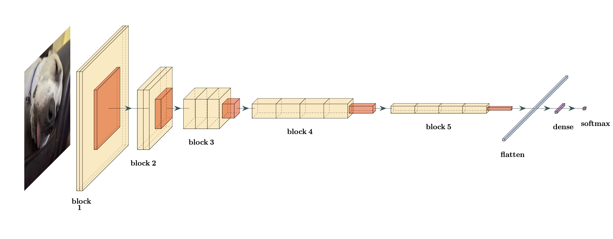
For example, Figure 1.3 shows a diagram of a type of deep learning model called a convolutional neural network that is often used for making predictions on images. It consists of several layers that manipulate the data. This particular model, dubbed VGG16, was proposed by Simonyan and Zisserman (2014).
The color image on the left is a data point. The first block has three layers. The two larger yellow boxes are convolutional layers. They move a small multidimensional array over the larger data array to compute localized features. For example, for an image that is 150 x 150 pixels, a convolution that uses a 3x3 filter will move this small rectangle across the array. At the (2,2) position, it takes the average of all adjacent pixel locations.
After the convolutional operations, a smaller pooling layer is shown in orange. Pooling, usually by finding the maximum feature value across different image regions, compresses/downsamples the larger feature set so a smaller size without diminishing features with large signals.
The next three blocks consist of similar convolutional and pooling layers but of different dimensions. The idea behind these blocks is to reduce the image data to a smaller dimension width/height dimension in a way that extracts potentially important hierarchical features from the image.
After block 5, the data are flattened into a single array, similar to the columns in a tabular data set. Up to this point, the network has been focused on preprocessing the image data. If our initial image were 150 pixels by 150 pixels, the flattening process would result in over 8 thousand predictors that would be used in a supervised ML model. The network would have over 14 million model parameters to estimate from the data to get to this point.
After flattening, the final two layers correspond to the classic supervised neural network model (Bishop 1995). The original paper used four large supervised neural network layers; for simplicity, Figure 1.3 shows a single dense layer. This can add dozens of millions of additional parameters for a modest-sized dense layer.
There are many types of deep learning models. Another example is recurrent neural networks, which create layers that are proficient at modeling data that occur in sequences such as time series data or sentences (i.e., a sequence of words).
Very sophisticated deep learning models have generated, by far, the best predictive ability for images and similar data. It would seem natural to think these models would be just as effective for tabular data. However, this has not been the case. Machine learning competitions, which are very different from day-to-day machine learning work, have shown that many other models can consistently do as well or likely better on tabular data sets. This has generated an explosion of literature7 and social media posts that try to explain why this is the case. For example, see Borisov et al. (2022) and McElfresh et al. (2023).
We believe that exceptionally complex DL models are handicapped in several ways when taken out of the environments where they have been successful.
First, the complexity of these models requires extreme amounts of data, and the constraints of such large data sets drive how the models are developed.
For example, keeping very large data sets in a computer’s memory is almost impossible. As discussed earlier, we use the data to find optimal values of our parameters for some objective functions (such as classification accuracy). Using traditional optimization procedures, this is very difficult if the data cannot be accessed simultaneously. Deep learning models use more modern optimization methods, such as stochastic gradient descent (SGD) methods, for estimating parameters. It does not simultaneously hold all of the data in memory and fits the model on small incremental batches of data. This is a very effective technique, but it is not an approach one would use with data set sizes that are more common (e.g., less than a million data points). SGD is less effective for smaller data sizes than traditional in-memory optimizers. Another consequence of huge data requirements is that model training can take an excruciatingly long time. As a result, efficient model development can require specialized hardware. It can also drive how models are optimized and compared. DL models are often optimized by sequentially adjusting the model. Other ML models can be optimized with a more methodical simultaneous design that is often more efficient, systematic, and effective than sequential optimizers used with deep learning.
Another issue with deep learning models is that their size and mathematical structure are associated with a very difficult optimization problem; their objective function is non-convex. We’d like to have an optimization problem that has some guarantees that a global optimal value exists (and can be found). That is often not the case for these models. For example, if we want to estimate the VGG16 model parameters with the goal of maximizing the classification accuracy for finding dogs in an image, it can be difficult to get a reliable estimate and, if we do, we don’t know if it is really the correct answer.
Because the optimization problem is so difficult, much of the user’s time is spent optimizing the model parameters or tuning the network structure to find the best results. When combined with how long it takes for a single model fit, deep learning models are very high maintenance compared to other models when used on tabular data. They can probably produce a model that is marginally better than the others, but doing so requires an inordinate amount of time, effort, and constraints. DL models are superior for certain hard problems with large data sets. For other situations, other ML models can go probably go further and faster8.
Finally, there are some data-centric reasons that the successfulness of deep learning models doesn’t automatically translate to tabular data. There are characteristics of tabular data that don’t often occur in stereotypical DL applications. For example:
- In some cases, a group of predictors might be highly correlated with one another. This can compromise some of the mathematical operations used to estimate parameters in neural networks (and many other models).
- Unless we have extensive prior experience with our data, we don’t know which are informative and which are irrelevant for predicting an outcome. As the number of non-informative predictors increases, the performance of neural networks decreases. See Section 19.1 of Kuhn and Johnson (2013).
- Predictors with “irregular” distributions, such as skewness or heavy tails, can harm performance (McElfresh et al. 2023).
- Missing predictor data are not naturally handled in basic neural networks.
- “Small” sample sizes or data dimensions with at least as many predictors as rows.
as well as others. These issues can be overcome by adding layers to a network designed to counter specific challenges. However, in the end, this ends up adding more complexity. We propose that there are a multitude of other models, and many of them are resistant or robust to these types of data-specific characteristics. It is better to have different tools in our toolbox; making a more complex hammer may not help us put a screw in a wall.
The deep learning literature has resulted in many collateral benefits for the broader machine learning field. We’ll describe a few techniques that have improved machine learning in subsequent chapters,
1.7 Modeling Philosophies
talk about subject-matter knowledge/intuition vs “let the machine figure it out”. biased versus unbiased model development.
assistive vs automated usage
1.8 Outline of These Materials
This work is organized into parts:
- Introduction: The next chapter shows an abbreviated example to illustrate important concepts used later.
- Preparation: These chapters discuss topics such as data splitting and feature engineering. These activities occur before the actual training of the machine learning model but are critically important.
- Optimization: To find the model that has the best performance, we often need to tune them so that they are effective but do not overfit. These chapters describe overfitting, methods to measure performance, and two different classes of optimization methods.
- Classification: Various models for classification are described in this part.
- Regression: These chapter describe models for numeric outcomes.
- Characterization: Once you have a model, how do you describe it or its predictions? How do you know when you should question the results of your model? We’ll address these questions in this part.
- Finalization: Post-modeling activities such as monitoring performance are discussed.
Before diving into the process of creating a good model, let’s have a short case study. The next chapter is designed to give you a sense of the overall process and illustrate important ideas and concepts that will appear later in the materials.
Chapter References
Bishop, C. 1995. Neural Networks for Pattern Recognition. Oxford: Oxford University Press.
Borisov, V, T Leemann, K Seßler, J Haug, M Pawelczyk, and G Kasneci. 2022. “Deep Neural Networks and Tabular Data: A Survey.” IEEE Transactions on Neural Networks and Learning Systems.
Boykis, V. 2023. “What Are Embeddings?” https://doi.org/10.5281/zenodo.8015028.
Engel, T, and J Gasteiger. 2018. Chemoinformatics : A Textbook . Weinheim: Wiley-VCH.
Goodfellow, I, Y Bengio, and A Courville. 2016. Deep Learning. MIT press.
Holmes, S, and W Huber. 2018. Modern Statistics for Modern Biology. Cambridge University Press.
Hvitfeldt, E, and J Silge. 2021. Supervised Machine Learning for Text Analysis in R. CRC Press.
Kuhn, M, and K Johnson. 2013. Applied Predictive Modeling. Springer.
Kuhn, M, and K Johnson. 2019. Feature Engineering and Selection: A Practical Approach for Predictive Models. CRC Press.
Leach, A, and V Gillet. 2003. An Introduction to Chemoinformatics. Springer.
McElfresh, D, S Khandagale, J Valverde, V Prasad, G Ramakrishnan, M Goldblum, and C White. 2023. “When Do Neural Nets Outperform Boosted Trees on Tabular Data?” arXiv.
Prince, S. 2023. Understanding Deep Learning. MIT press.
Sanderson, B. 2017. Oathbringer. Tor Books.
Simonyan, K, and A Zisserman. 2014. “Very Deep Convolutional Networks for Large-Scale Image Recognition.” arXiv.
Yu, W, HK Lee, S Hariharan, WY Bu, and S Ahmed. 2007. “CCDB:6843, Mus Musculus, Neuroblastoma.”
Non-tabular data are later in this chapter.↩︎
This is a linear regression model.↩︎
This is a smaller version of a larger image that is 1392 pixels by 1040 pixels.↩︎
The original image would produce 2,895,360 flattened features.↩︎
Also known as “discrete” or “nominal” data.↩︎
A note to readers: these
?sec-*references are to sections or chapters that are planned by not (entirely) written yet. They will resolve to actual references as we add more content.↩︎To be honest, the literature in this area has been fairly poor (as of this writing).↩︎
That said, simple neural network models can be very effective. While still a bit more high maintenance than other models, it’s a good idea to give them a try (as we will see in the following chapter).↩︎